Understanding our Data
The data set below is a selection from this larger dataset (link here) of songs from the year 2000 on Billboard’s top 100.
| year | artist_inverted | track | time | genre | date_entered | date_peaked | x1st_week | … | x53rd_week | x54th_week | x55th_week | x56th_week | x57th_week | x58th_week | x59th_week | x60th_week |
|---|---|---|---|---|---|---|---|---|---|---|---|---|---|---|---|---|
| 2000 | Lonestar | Amazed | 4:25 | Country | 1999-06-05 | 2000-03-04 | 81 | … | 20.0 | 22.0 | 22.0 | 25.0 | 26.0 | 31.0 | 32.0 | 37.0 |
| 2000 | Creed | Higher | 5:16 | Rock | 1999-09-11 | 2000-07-22 | 81 | … | 17.0 | 17.0 | 21.0 | 26.0 | 29.0 | 32.0 | 39.0 | 39.0 |
| 2000 | 3 Doors Down | Kryptonite | 3:53 | Rock | 2000-04-08 | 2000-11-11 | 81 | … | 49.0 | NaN | NaN | NaN | NaN | NaN | NaN | NaN |
| 2000 | Creed | With Arms Wide Open | 3:52 | Rock | 2000-05-13 | 2000-11-11 | 84 | … | NaN | NaN | NaN | NaN | NaN | NaN | NaN | NaN |
| 2000 | Hill, Faith | Breathe | 4:04 | Rap | 1999-11-06 | 2000-04-22 | 81 | … | 47.0 | NaN | NaN | NaN | NaN | NaN | NaN | NaN |
The data tracks the date a song entered the Billboard Top 100 and the weekly position it had there after. NaN is used to represent the weeks when a song has either not reached the chart yet, or has fallen off the chart for that week(s).
I would like to see which songs had the longest runs on the chart. Or in other words which songs have the most numerical values in ‘x_weeks’ columns. The easiest way to do this in Pandas is to add a new column to our data frame that we can call ‘week_count’.
# First we can grab a data frame of just the weeks to make things a little easier to work with.
df_weeks = df[list(filter(lambda x: x.startswith('x'), df.columns))].transpose()

# We can now transpose the dataframe and count. The index will still match, so we can tack it on with a new name.
df['weeks_on_chart'] = [int(c) for c in df_weeks.count()]
# I also need to convert the counts to ints

#Let's sort our dataframe and look at what the longest running song was
top_5 = df.sort_values('weeks_on_chart', ascending=False).head()
What does our output look like?
| artist_inverted | track | genre | weeks_on_chart |
|---|---|---|---|
| Creed | Higher | Rock | 57 |
| Lonestar | Amazed | Country | 55 |
| 3 Doors Down | Kryptonite | Rock | 53 |
| Hill, Faith | Breathe | Rap | 53 |
| Creed | With Arms Wide Open | Rock | 47 |
Oh man, 2000 wasn’t exactly the greatest year for music. But nonetheless, there is still plenty of things for us to explore. What did these long runs on the chart look like? Did any of these songs reach number one? If so for how long? There a lot of questions I’d like to have answered, but don’t feel like typing all those things out.
This calls for a visualization!
Visualizing our Data
Plotting with pandas can be incredibly simple, especially when we have a well organized dataframe. To plot the runs of the top 5 songs we only need a few lines of code.
# First we need to import some plotting libraries
import matplotlib.pyplot as plt
import seaborn as sns
# And then we make our plot!
df_weeks[top_5.track].plot(style='-')
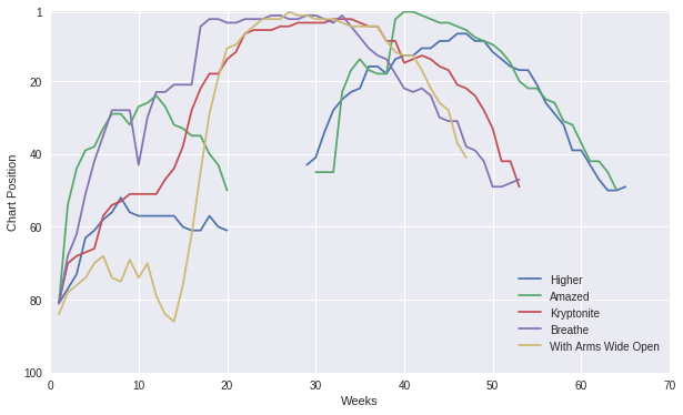
This answers many of my earlier questions, but this plot is still a bit deceptive. The x axis of this plot represents the week a song entered the top 100; meaning every song’s run starts at week one. However, each song on the chart has a different literal week of the year 2000 for its week one, meaning the start date for ‘Higher’ is a different week one than the start date for ‘Amazed’. Our current plot does not show this. Additionally, there is a visible gap between weeks 20 and 40. After examining this phenomena I learned that the dataset being used for these plots is apparently corrupted. A large portion of the values between the columns xWeek20 and xWeek40 are totally missing.
If we were to somehow translate our x axis to actual dates we could make the plot I really want to see and simultaneously allow ourselves to examine what rankings are missing from the chart for a given week. We could infer our missing data by iterating over each week in the year 2000 and find what rankings from the top 100 are missing.
In order to do this we are going to have to work with Timeseries. But I will save that analysis for next time…