Introduction
The motivation for this project came from my own personal struggles with procrastination. There exist many productivity apps out there to help people like me stay focused despite the seemingly infinite number of distractions that exist on the current state of the Internet (cough Reddit cough). The problem is, most of these productivity apps block website purely off URL. In many cases this is good enough, but often times blocking an entire URL creates more problems than it solves. Youtube, for example, is one of the largest sources of distraction the Internet has to offer. Naturally, it is a website one would block when they would like to be productive. However, Youtube also provides a vast wealth of incredibly informative videos. There have been numerous times when watching a five minute video on matrix multiplication to refresh my memory would lead to hours of increased productivity down the line. But alas, the site is blocked by my supposedly helpful productivity app. So I find myself in at a crossroads: I can disable the app to watch the video I want to see, but run the risk of spiraling down a never ending path of cat videos; or I leave the app running and search for a less effective refresher. I should not have to choose. So I set out to find a better way.
Let’s start by importing our data
import pandas as pd
import numpy as np
import matplotlib.pyplot as plt
import seaborn as sns
from sklearn import model_selection
from sklearn import linear_model
from sklearn import ensemble
from sklearn.metrics import accuracy_score, precision_score, recall_score, confusion_matrix, classification_report
from sklearn.linear_model import LogisticRegression
from sklearn.pipeline import Pipeline

%matplotlib inline

data = pd.read_csv('parsed_html.csv')
X = data[['text','url']]

# Splitting our data into a training and test set before we begin our data building
X_train, X_test, y_train, y_test = model_selection.train_test_split(data, data.activity,test_size=0.33, random_state=43)
Model building
Building a grid searched pipeline
I am using a grid search over a pipeline to find the best model to use. After much trial and error I settled on a logistic regression model. First off it simply performaned the best. But additionally it is by far the most interpretible model. Also, Lasso Regularization is a great way to reduce the number of features generated by the countvectorization process, and the use of ngrams. At one point I had a dataframe with over 2,000,000 features. Lasso Regularization reduced that to a few hundred.
from nltk.corpus import stopwords
from sklearn.model_selection import GridSearchCV
from sklearn.feature_extraction.text import CountVectorizer, HashingVectorizer, TfidfVectorizer, TfidfTransformer

# Let's create some stop words. I chose these values after doing a little bit of EDA.
stop = stopwords.words('english')
stop = stop + ['https', 'www', 'com', 'http']
cvt = CountVectorizer(stop_words=stop, ngram_range=[1,4])

# Here we are initializing the values we want to grid search over.
param_grid = dict(vect = [CountVectorizer()],
                  vect__ngram_range=[[1,3],[1,4]], # Trying different ngram ranges
                  vect__stop_words = [stop],
                tfidf = [TfidfTransformer()],
                tfidf__norm = [None],
                clf=[LogisticRegression()],
                clf__C=[.04,.1,.06, .07, .05], # Trying different coefficients for alpha
                clf__penalty=['l1'])


pipeline = Pipeline([
    ('vect', cvt),
    ('tfidf', TfidfTransformer(norm=None)),
    ('clf', LogisticRegression(penalty='l1'))
])

grid_search = GridSearchCV(pipeline, param_grid=param_grid)

grid_search.fit(X_train.text, y_train)
Analyzing our results
Calculating some metrics
# Finding our best pipeline and pulling out the useful components
pipeline = grid_search.best_estimator_
lm =  pipeline.named_steps['clf']
vect = pipeline.named_steps['vect']

# Let's see what our accuracy looks like
grid_search.best_estimator_.score(X_test.text, y_test)
Out: 0.97214484679665736
Our accuracy score is looking great. 97.5% is great, but we should compare it to our baseline distribution before we get to excited.
# Caluclating our baseline
(y_train == 'work').sum()/float(len(y_train))
out: 0.41483516483516486
So we have massively improved over random chance. This is a good start. We should look at some additional metrics as well to see if we have anything to be concerned about.
result_x = vect.transform(X_test.text)

pred = lm.predict(result_x)
print(classification_report(y_test, pred))
precision    recall  f1-score   support

procr       0.96      0.98      0.97       214
work       0.97      0.94      0.95       145

avg / total       0.96      0.96      0.96       359
So far so good. I don’t see anything that looks particularly concerning with these results. Our recall being a little less for work then procrastination is something to keep in mind going forward. We may want to consider examining our predict probabilities to see what kind of values are getting misclassified.
Next we should take a look at our ROC and the area under the curve.
from sklearn.metrics import roc_curve, auc
# Here is some helpful code found on stack overflow
pred_proba = lm.predict_proba(result_x)
fpr, tpr, threshold = roc_curve(y_test == 'work', pred_proba[:,1])
roc_auc = auc(fpr, tpr)

plt.figure(figsize=(20,10), dpi=80)
plt.title('Receiver Operating Characteristic', fontsize=22);
plt.plot(fpr, tpr, 'b', label = 'AUC = %0.3f' % roc_auc);
plt.legend(loc = 'lower right', fontsize=20);
plt.plot([0, 1], [0, 1],'r--');
plt.xlim([0, 1]);
plt.ylim([0, 1]);
plt.ylabel('True Positive Rate', fontsize=18);
plt.xlabel('False Positive Rate', fontsize=18);
plt.xticks(fontsize=14)
plt.yticks(fontsize=14)
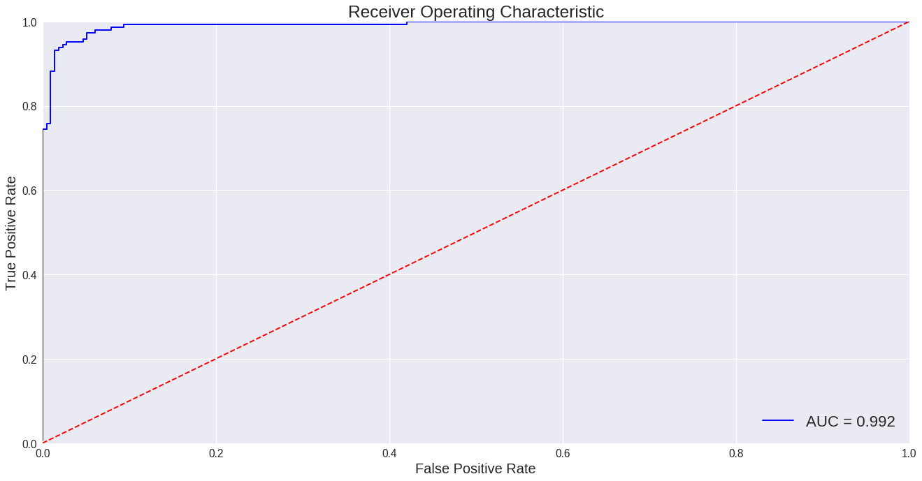
Wow! 0.992 AUC_ROC. That is amazing. I think we can safely say we have created an extremely effective model for predicting procrastination.
Taking a deeper look at our features
# This bit of code is pulling out my features that have coefficients greater than zero
# Lasso regularization reduces the coef to 0 of the features (in our case unique ngrams)
import math
features =(vect.get_feature_names())
feature_dict = {}
for (i, f) in enumerate(features):
    if np.abs(lm.coef_[0][i]) > 0:
        feature_dict[f] = lm.coef_[0][i]

# For convienence sake I'll put the features into a data frame for easier exploration
feature_df = pd.DataFrame.from_dict(feature_dict, orient='index')
feature_df.columns = ['coef']
Let’s take a quick look at the number of features and our total documents. We really do not want a model utilizing more features than we have documents. Our reguralization should have accounted for this, but it’s not a bad idea to double check.
# How many documents do I have in my training set
print("Number of docs: " + str(len(X_train)))

# How many features do I have after reguralization
print("Number of features: " + str(len(feature_df)))
Number of docs: 728
Number of features: 211
# We can raise our logisitic regression coef to the e to calculate the odds ratio
feature_df['odds_ratio'] = feature_df['coef'].apply(np.exp)
Now let’s look at what words are most associated with procrastination and productivity. We can sort our dataframe by odds ratio. The smaller odds ratio means words that are less related productivity, and a higher ratio means more related.
feature_df.sort_values('odds_ratio').head(10)
| coef | odds_ratio | |
|---|---|---|
| game | -0.130174 | 0.877943 |
| likes | -0.093046 | 0.911152 |
| thwas | -0.087130 | 0.916558 |
| -0.074749 | 0.927976 | |
| photo | -0.072818 | 0.929770 |
| ignore_index | -0.056659 | 0.944916 |
| attack | -0.054527 | 0.946933 |
| video | -0.043512 | 0.957421 |
| src | -0.042894 | 0.958013 |
| us | -0.040551 | 0.960260 |
feature_df.sort_values('odds_ratio',ascending=False).head(10)
| coef | odds_ratio | |
|---|---|---|
| github | 0.203852 | 1.226116 |
| using | 0.162867 | 1.176880 |
| data | 0.089620 | 1.093759 |
| code | 0.080694 | 1.084039 |
| file | 0.079490 | 1.082735 |
| import | 0.069770 | 1.072262 |
| 0.065247 | 1.067422 | |
| friction | 0.061906 | 1.063863 |
| project euler | 0.058094 | 1.059814 |
| stack | 0.049860 | 1.051124 |
Looking at the top 10 words related to procrastinating I can see a lot of things that make sense. Words like ‘game’, ‘reddit’, ‘photo’ make sense in a general sense. ‘5e’ and ‘attack’ look related to Dungeons and Dragons (I thing I spend a lot of time reading about). ‘src’, ‘us’, and ‘thwas’ I don’t undrestand as much.
The top 10 words for being productive are almost all really clear to me. ‘github’ being the strongest indicator comes at no surprise, with ‘data’, ‘file’, ‘code’, and ‘import’ all following closely behind. The word ‘using’ is interesting. I do find myself googling phrases like “classifying data using logistic regression’ quite frequently, perhaps that verb is largely prevalent in sentences for when I’m being productive. ‘instagram’ is another interesting word. I do not use instagram. I don’t even have an account. But I did spend a long afternoon one day trying to figure out how to get their API to work for a project I was working on. ‘Kurzgesagt’ is the name of a Youtube channel for educational videos. I am extremely please to see it show up as an indicator of productivity. That is a text book example of the kind of key word I was hoping to find that would distinguish mindless Youtube videos from educational ones.